Use Case: Keeping an ML Model in the Loop

The demo Real-time feature engineering computes the inputs an ML model needs. This article shows how a real-time Feldera pipeline can interact with a model, feeding it data, reading the predictions back, and measuring how good the predictions are, while the pipeline keeps running.

Calling a model from a user-defined function generally won't work, because UDFs in Feldera must be fully deterministic functions. In this article the model runs as a separate process outside the pipeline, and the two exchange data through a view (which supplies the model's inputs) and a table (which supplies the model's outputs).

The full SQL for the pipeline is in model_scoring.sql. A mock model server that closes the loop, and drives the whole lifecycle, is in test_model_scoring.py.

The pattern

• Feature extraction is expressed in SQL. fingerprinted_features is the resulting set of model inputs: one row per feature vector.
• unpredicted_features narrows the requests to requests that have received no prediction answers yet. This is the view the model server subscribes to.
• The server runs the model and writes model outputs into the model_prediction table. It only ever inserts; the model is stateless.
• The pipeline reads that table like any other input and scores the predictions against ground truth as it arrives (possibly much later).

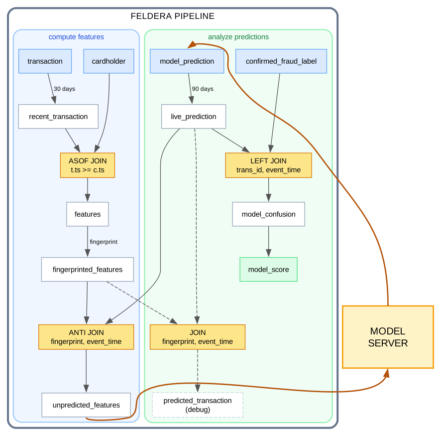
Input data

There are 2 main input tables:

• cardholder holds information about credit card holders. Notice that the primary key of this table contains a unique ID but also a timestamp. This essentialle makes cardholders versioned
• transaction holding information about credit card transaction. This models an append-only stream of transactions which are never deleted

There is an additional table confirmed_fraud_label, which is expected to be populated much later than these two tables, which indicates transactions that were determined later to be fraudulent. This information is used to determine how good the predictions from a model were.

Enrichment

Enriched data is produced by joining recent_transaction and cardholder using an ASOF JOIN, which selects the version in effect when the event happened rather than the version current now. recent_transaction is transaction restricted to the prediction window, so the join never sees the whole history:

FROM recent_transaction t
LEFT ASOF JOIN cardholder c
MATCH_CONDITION ( t.ts >= c.ts )
ON t.cc_num = c.cc_num

Fingerprinting request for the model server

For every request the model server has to produce a prediction. When providing a prediction, the model server has to describe which feature the score corresponds to. For this purpose, requests to the model are identified by a fingerprint including every feature value:

CREATE MATERIALIZED VIEW fingerprinted_features AS
SELECT
    MD5(CAST(f.trans_id AS VARCHAR) || '|' ||
        CAST(f.ts AS VARCHAR) || '|' ||
        CAST(f.amount AS VARCHAR) || '|' ||
        f.merchant_category || '|' ||
        CAST(f.zip AS VARCHAR) || '|' ||
        CAST(f.credit_limit AS VARCHAR) || '|' ||
        CAST(f.pct_of_limit AS VARCHAR) || '|' ||
        CAST(f.avg_amount_7d AS VARCHAR) || '|' ||
        CAST(f.txn_count_7d AS VARCHAR)) AS request_fingerprint,
    f.*
FROM features f
WHERE f.ts > NOW() - INTERVAL 30 DAYS;

warning

Every feature the model reads must appear in the fingerprint. A feature left out lets a stale prediction survive a change to it.

The work queue between the pipeline and the model

A model server should hold no state. We keep the outstanding in the view unpredicted_features: a request is pending when no prediction for it exists.

CREATE MATERIALIZED VIEW unpredicted_features AS
SELECT r.*
FROM fingerprinted_features r
WHERE NOT EXISTS (
    SELECT 1 FROM live_prediction p
    WHERE p.request_fingerprint = r.request_fingerprint AND p.event_time = r.ts);

The server subscribes to unpredicted_features over HTTP egress with send_snapshot=true, which replays the outstanding set on connect. A reconnect therefore resumes where it left off.

We use backpressure=true in this demo; this prevents the pipeline from producing requests faster than the model can serve.

HTTP or Kafka

This demo uses HTTP so that it does not need to run additional services. In production we would attach a Kafka output connector to unpredicted_features instead, and the model server would consume the topic:

CREATE MATERIALIZED VIEW unpredicted_features
WITH ('connectors' = '[{
    "transport": {
        "name": "kafka_output",
        "config": { "bootstrap.servers": "...", "topic": "prediction-requests" }
    },
    "format": { "name": "json", "config": { "update_format": "insert_delete" } }
}]')
AS ...

The two differ in ways that matter:

	HTTP egress	Kafka
Fault tolerance	none	supported
Connector lifetime	created on connect, deleted on disconnect	declared, persistent
If the server is down	requests emitted meanwhile are missed	they wait in the topic
Backpressure	backpressure=true blocks the pipeline	none; the queue absorbs the backlog
Recovery on restart	send_snapshot=true replays the outstanding set	resume from the consumer offset

Using HTTP, a model server that disconnects loses whatever was emitted while it was away, and only reconnecting with send_snapshot=true recovers it.

In this write-up the model server sends predictions to the pipeline hrough HTTP ingress; in production model_prediction could declare a Kafka input connector, which is also fault-tolerant, and the server would append to that topic instead of posting:

CREATE TABLE model_prediction (
    ...
) WITH ('connectors' = '[{
    "transport": {
        "name": "kafka_input",
        "config": { "bootstrap.servers": "...", "topic": "predictions",
                    "start_from": "earliest" }
    },
    "format": { "name": "json", "config": { "update_format": "insert_delete" } }
}]');

Using Kafka in both directions makes the whole loop durable and the pipeline and he model fully decoupled: neither has to be running for the other to make progress, and neither talks the other directly. Replays are harmless because model_prediction has a primary key, so a redelivered prediction upserts rather than duplicating.

The only way the pipeline SQL needs to change is by adding the connector declarations.

Finite-state design

Nothing in this design retains data indefinitely, even though the input tables may grow indefinitely.

• LATENESS bounds the state for both transaction and cardholder.

• A temporal filter bounds the contents:

WHERE f.ts > NOW() - INTERVAL 30 DAYS

This ensures that all views that hold features only contain data from the last 30 days.

LATENESS and the temporal filter serve complementary purposes (how Feldera garbage collects old state):

Horizon	Question
30 days, temporal filter on fingerprinted_features	how far back is it worth predicting?
90 days, LATENESS on predictions	how long can ground truth take to arrive?

Predictions produced by the model must be retained longer than the original requests, allowing the ground truth to arrive delayed.

When the model server is started it produces immediately for the pipeline data for the prediction window (last 30 days), rather than only scoring new traffic. This enables the pipeline to evaluate the quality of the model immediately, without waiting for 90 days.

model_prediction receives data written by the model. In our implementation the model server uses http to write to this table. The table has a primary key so that it holds one current answer per transaction:

CREATE TABLE model_prediction (
    event_time TIMESTAMP NOT NULL LATENESS INTERVAL 90 DAYS,
    request_fingerprint VARCHAR NOT NULL,
    trans_id BIGINT NOT NULL,
    fraud_probability DECIMAL(5, 4) NOT NULL,
    predicted_at TIMESTAMP NOT NULL,
    PRIMARY KEY (event_time, trans_id)
);

Scoring the model

Ground truth usually arrives long after the prediction, and for most events it may never arrive at all: only a small fraction of transactions are discovered to be fraudulent. We treat by default a missing transaction label as a negative (a transaction with no ground truth is assumed to be non fraudulent):

The confusion matrix is computed using a left join of the ground truth and the predictions. Precision and recall are estimated from these counts. DIV_NULL returns NULL instead of failing when the denominator is zero, so it is handy for the case when a model has predicted no fraud at all:

CREATE MATERIALIZED VIEW model_score AS
SELECT
    scored,
    true_positive,
    false_positive,
    false_negative,
    DIV_NULL(CAST(true_positive AS DECIMAL(12, 6)),
             true_positive + false_positive) AS precision_score,
    DIV_NULL(CAST(true_positive AS DECIMAL(12, 6)),
             true_positive + false_negative) AS recall_score
FROM model_confusion;

The CAST is used because otherwise the computation uses integer division.

One model at a time

This demo scores a single model. Nothing in the pipeline verifies that a model server is running: if none is, requests accumulate unanswered in unpredicted_features until they fall out of the prediction window.

Running several models at once is possible, not shown here. It could be implemented by having an additional table listing all deployed model versions.